Inertial Delay

We can add delays to assign statements to simulate gate delays. This has the effect of delaying the assign statement a few nanoseconds, but with one caveat: inertial delay. Input pulses shorter than the specified delay are filtered out.
This concept is best explained with an example. Consider this simulation:
`timescale 1ns / 1ps
module inertial_delay;

// inputs
reg X;

// outputs
wire [4:0] Y;

assign Y[0] = X;        // 0 ns delay
assign #1 Y[1] = X;     // 1 ns delay
assign #2 Y[2] = X;     // 2 ns delay
assign #3 Y[3] = X;     // 3 ns delay
assign #4 Y[4] = X;     // 4 ns delay

initial begin
    X = 0;
    #10 X = 1;
    #2 X = 0;  // create 2 ns pulse (high at 10 ns, low at 12 ns)
    #10 $finish;
end
endmodule
What would be the expected outcome of Y[4:0]? X is a signal with a 2 ns pulse. Take a moment to predict what Y[0], Y[1], Y[2], Y[3], and Y[4] will look like.
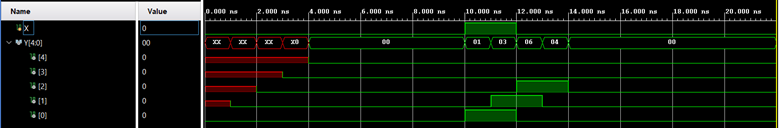
Does this result surprise you? Notice how the 3 and 4 ns delays filtered out the pulse! This is inertial delay. Consider this second example. Can you predict what Y[4:0] will look like?
`timescale 1ns / 1ps
module inertial_delay_2;

// inputs
reg A, B;

// outputs
wire [4:0] Y;

assign    Y[0] = A & B;
assign #1 Y[1] = A & B;     // 1 ns delay
assign #2 Y[2] = A & B;     // 2 ns delay
assign #3 Y[3] = A & B;     // 3 ns delay
assign #4 Y[4] = A & B;     // 4 ns delay

initial begin
    A = 1; B = 1;
    #10 A = 0; B = 1;
    #1  A = 1; B = 1;
    #1  A = 1; B = 1;
    #1  A = 0; B = 1;
    #1  A = 0; B = 0;
    #1  A = 1; B = 0;
    #1  A = 1; B = 1;
    #10 $finish;
end
endmodule
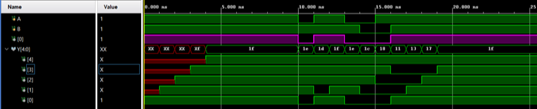
There is a lot going on here. This problem become easier if we look at the waveform Y[0] = A & B, shown in magenta.
![Figure 2. Y[0] = A & B](/img/a640a3bd4715c5249828e35ed8567930.png)
There are two negative pulses: a 1ns pulse at t=10ns, and a 3ns pulse at t=13ns. Take a moment to visualize what Y[4:0] looks like. Draw it out on paper before looking at the answer. Start with Y[0] (given) and work through Y[4].
Inertial delay will appear throughout this lab. Use it to explain why some glitches persist, while other glitches vanish in various circuits.